Clustering Hitters by their Distribution of Batted Balls
Grouping similar baseball players is essential to teams. It could allow a larger sample size when predicting batter vs. pitcher matchups or reduce the amount of information needed on a scouting report.
There are a variety of possible metrics by which to cluster hitters, but I will focus on just two: the exit velocity and launch angle of their batted balls. I focus on these two characteristics of batted balls because by knowing a ball’s exit velocity and launch angle, you know what the probable result of the play is.
Because a batter will hit hundreds of balls throughout the season, each with their own exit velocity and launch angle, it can be tricky to summarize the information in a way that is useful for producing clusters. I could sample statistics, such as max exit velocity, average exit velocity, average launch angle, or proportion of batted balls that fall in a certain range of exit velocity and launch angle, but these numbers fail to capture the complexity that is a batter’s entire distribution of batted balls. For example, the below figure shows the bivariate distribution of exit velocity and launch angle for four players, as well as their average exit velocity and launch angle (the red dot). Although the four players vary in the hitting style and prowess, the difference between their averages is much less stark than the difference between their distributions.
library(MASS)
library(tidyverse)
source("dbcon.R")
set.seed(101)
in_play <- dbGetQuery(con, "select * from bayes_project")

in_play <- in_play %>%
  dplyr::select(player_name, launch_speed, launch_angle) %>%
  na.omit()

ggplot() +
  geom_density2d_filled(in_play %>%
                          filter(player_name %in% c("Mike Trout",
                                                    "Omar Narvaez",
                                                    "Freddie Freeman",
                                                    "David Dahl")),
                        mapping = aes(x=launch_speed,
                                      y = launch_angle),
                        bins = 50, alpha = .8, na.rm = TRUE) +
  geom_point(in_play %>%
                group_by(player_name) %>%
                filter(player_name %in% c("Mike Trout", "Omar Narvaez",
                            "Freddie Freeman", "David Dahl")) %>%
                 summarize(mean_ev = mean(launch_speed),
                           mean_la = mean(launch_angle)),
               mapping = aes(x = mean_ev, y = mean_la), col = "red", size = 4, na.rm = TRUE) +
  facet_wrap(~player_name) +
  theme_light() +
  theme(legend.position = "none") +
  labs(x = "Exit Velocity", y = "Launch Angle", title = "Distributions vs. Means") +
  scale_x_continuous(limits = c(50, 120)) +
  scale_y_continuous(limits = c(-60,60))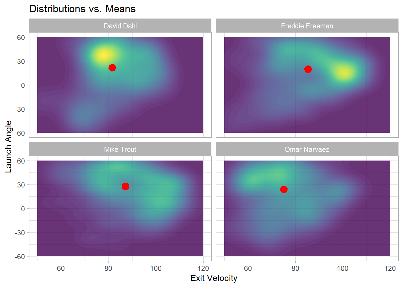
The idea behind clustering is to group similar things together and separate dissimilar things. In this case, I want to group hitters with similar batted ball distributions together. There are two problems with this. First, I need to approximate the distribution of batted balls for each player. This distribution will be irregular, so I will use 2-D kernel density estimation at a fine grid of points after standardizing the data.
in_play <- in_play %>%
  group_by(player_name) %>%
  filter(n() >= 100) %>%
  ungroup()

mean_ev <- mean(in_play$launch_speed)
sd_ev <- sd(in_play$launch_speed)
mean_la <- mean(in_play$launch_angle)
sd_la <- sd(in_play$launch_angle)

in_play <- in_play %>%
  mutate(launch_speed = (launch_speed-mean_ev)/sd_ev,
         launch_angle = (launch_angle-mean_la)/sd_la)

#for(k in 1:100){
players <- sort(unique(in_play$player_name))

get_density_estimate <- function(i){
  dat <- in_play %>%
    filter(player_name == players[i]) %>%
    dplyr::select(launch_speed, launch_angle)

  dens <- kde2d(dat$launch_speed, dat$launch_angle, n = 50, lims = c(-4,4,-4,4))$z %>%
    as.vector()

  dens
}


dists <- sapply(1:length(players), get_density_estimate)
The second issue is in defining a distance/similarity metric for entire distributions. I will use a modified version of Kullback-Leibler (KL) divergence. For continuous distributions \(P\) and \(Q\) with densities \(p(x)\) and \(q(x)\) respectively, the KL divergence is defined as \[D(P|Q) = \int_{-\infty}^{\infty} p(x) \text{log}\left(\frac{p(x)}{q(x)}\right)dx.\]
Because there is no known equation for the continuous probability density function of each distribution, but instead there are density estimates at \(N\) locations, \(a_1,...,a_{N}\), an adjustment must be made. Since the grid with the locations of the density estimates is the same for each distribution (ensuring the densities are on the same scale), I will adjust to \[D(P|Q) = \sum_{i=1}^{N} p(a_i) \text{log}\left(\frac{p(a_i)}{q(a_i)}\right).\]
KL divergence is not a symmetric measure, so to incorporate it into the clustering algorithm, I instead use \(d(P,Q) = D(P|Q) + D(Q|P)\).
After approximating the distribution for each player and calculating the distances between each distribution, I can check to see which players are closest together. For example, below I show the five players with the closest batted ball distribution to Mike Trout.
dist_mat <- matrix(NA, length(players), length(players))
for(i in 1:length(players)){
  for(j in 1:length(players)){
    if(i != j){
      dist_mat[i,j] <- sum(dists[,i]*log(dists[,i]/dists[,j])) +
        sum(dists[,j]*log(dists[,j]/dists[,i]))
    }
  }
}

colnames(dist_mat) <- players
rownames(dist_mat) <- players

dist_mat["Mike Trout",] %>%
  sort() %>%
  head(5)
## Trevor Story Alex Dickerson Brandon Belt Nolan Arenado Will Smith
## 7.703614 9.064337 9.613870 9.784453 10.182298Using the distances between all pairs of distributions, I use an agglomerative clustering algorithm to put the distributions into clusters, grouping the clusters that are closest together in an iterative process. Starting with \(n\) clusters (with one player per cluster), I combine the two clusters that have the smallest distance between them to form \(n-1\) clusters. I then combins the two closest clusters and repeat the process until reaching the desired number of clusters. Because I have the distance between distributions, rather than between clusters, I use Ward’s linkage to combine the clusters. Ward’s linkage combines clusters to minimize the total sum of squares error (squared distance from each distribution to its cluster mean). For this project, I arbitrarily stop at 20 clusters because it seems like a reasonable number of batted ball profiles to exist.
dc <- dist(dist_mat)
wardlink <- hclust(dc,method='ward.D2')
kl_clusters <- cutree(wardlink,20) %>%
  as.data.frame() %>%
  rownames_to_column("player") %>%
  rename(player_name = player, cluster = '.') %>%
  arrange(cluster)
Describing the 20 clusters is a bit of a challenge. One way to do it is to show where the players in each cluster fall in certain outcome statistics. Below, using data obtained from FanGraphs, I show where players in each of the 20 clusters fall in Batting Average on Balls in Play, or BABIP, and in Home Runs per Fly Ball (HR/FB). I chose to display these two statistics because they represent the ability to hit for average and power, two traditional hitting tools. I also highlight some of the more notable players in baseball.
advanced <- read.csv("advanced_2020.csv")
batted_ball <- read.csv("batted_ball_2020.csv")
statcast <- read.csv("statcast_2020.csv")

advanced <- advanced %>%
  janitor::clean_names() %>%
  mutate(bb = as.numeric(str_remove(bb, "%")),
         k = as.numeric(str_remove(k, "%"))) %>%
  dplyr::select(player_name = i_name,
         bb_perc = bb,
         k_perc = k,
         avg,
         obp,
         slg,
         babip,
         woba = w_oba,
         wrc_plus = w_rc_2
         ) %>%
  mutate(player_name = case_when(player_name == "Giovanny Urshela" ~ "Gio Urshela",
                                 player_name == "A.J. Pollock" ~ "AJ Pollock",
                                 player_name == "Shed Long" ~ "Shed Long Jr.",
                                 player_name == "Yoshitomo Tsutsugo" ~ "Yoshi Tsutsugo",
                                 player_name == "Cedric Mullins II" ~ "Cedric Mullins",
                                 player_name == "Dee Gordon" ~ "Dee Strange-Gordon",
                                 player_name == "D.J. Stewart" ~ "DJ Stewart",
                                 player_name == "Nicholas Castellanos" ~ "Nick Castellanos",
                                 TRUE ~ player_name))

batted_ball <- batted_ball %>%
  janitor::clean_names() %>%
  mutate(gb = as.numeric(str_remove(gb, "%")),
         fb = as.numeric(str_remove(fb, "%")),
         hr_fb = as.numeric(str_remove(hr_fb, "%")),
         ifh_2 = as.numeric(str_remove(ifh_2, "%")),
         pull = as.numeric(str_remove(pull, "%")),
         oppo = as.numeric(str_remove(oppo, "%")),
         soft = as.numeric(str_remove(soft, "%")),
         hard = as.numeric(str_remove(hard, "%"))) %>%
  dplyr::select(player_name = i_name,
         gb, fb, hr_fb, inf_h = ifh_2, pull, oppo, soft, hard) %>%
  mutate(player_name = case_when(player_name == "Giovanny Urshela" ~ "Gio Urshela",
                                 player_name == "A.J. Pollock" ~ "AJ Pollock",
                                 player_name == "Shed Long" ~ "Shed Long Jr.",
                                 player_name == "Yoshitomo Tsutsugo" ~ "Yoshi Tsutsugo",
                                 player_name == "Cedric Mullins II" ~ "Cedric Mullins",
                                 player_name == "Dee Gordon" ~ "Dee Strange-Gordon",
                                 player_name == "D.J. Stewart" ~ "DJ Stewart",
                                 player_name == "Nicholas Castellanos" ~ "Nick Castellanos",
                                 TRUE ~ player_name)) %>%
  mutate(player_name = case_when(player_name == "Giovanny Urshela" ~ "Gio Urshela",
                                 player_name == "A.J. Pollock" ~ "AJ Pollock",
                                 player_name == "Shed Long" ~ "Shed Long Jr.",
                                 player_name == "Yoshitomo Tsutsugo" ~ "Yoshi Tsutsugo",
                                 player_name == "Cedric Mullins II" ~ "Cedric Mullins",
                                 player_name == "Dee Gordon" ~ "Dee Strange-Gordon",
                                 player_name == "D.J. Stewart" ~ "DJ Stewart",
                                 player_name == "Nicholas Castellanos" ~ "Nick Castellanos",
                                 TRUE ~ player_name))


kl_plot <- kl_clusters %>%
  left_join(advanced, by = "player_name") %>%
  left_join(batted_ball, by = "player_name") %>%
  na.omit() %>%
  mutate(keep_name = ifelse(player_name %in% c("Mike Trout", "Freddie Freeman",
                                               "Fernando Tatis Jr.", "Mookie Betts",
                                               "Aaron Judge", "Jose Abreu", "Manny Machado",
                                               "DJ LeMahieu", "Nelson Cruz", "Tim Anderson",
                                               "Juan Soto", "Marcell Ozuna", "Trea Turner",
                                               "Bryce Harper", "Ronald Acuna"),
                            TRUE, FALSE)) %>%
  mutate(avg_babip = mean(babip),
         avg_hr_fb = mean(hr_fb)/100)


ggplot() +
  geom_point(filter(kl_plot, !keep_name), mapping = aes(x=babip, y = hr_fb/100), alpha = .5) +
  geom_point(filter(kl_plot, keep_name) %>% arrange(player_name), mapping = aes(x=babip, y = hr_fb/100,
                                                       fill = player_name, shape = player_name), size = 4, alpha = .8) +
  geom_vline(xintercept = kl_plot$avg_babip[1]) +
  geom_hline(yintercept = kl_plot$avg_hr_fb[1]) +
  scale_shape_manual(name = "Player", values = c(21:25,21:25,21:25),
                     labels = filter(kl_plot, keep_name) %>% arrange(player_name) %>%  pull(player_name)) +
  scale_fill_manual(name = "Player", values = c(2:8, 10:16),
                    labels = filter(kl_plot, keep_name) %>% arrange(player_name) %>% pull(player_name)) +
  facet_wrap(~cluster) +
  theme_light() +
  labs(x = "BABIP", y = "HR/FB") +
  scale_y_continuous(labels = scales::percent_format(accuracy = 2)) +
  scale_x_continuous(breaks = c(".200" = .2, ".300"= .3, ".400" = .4)) +
  theme(text = element_text(size = 12))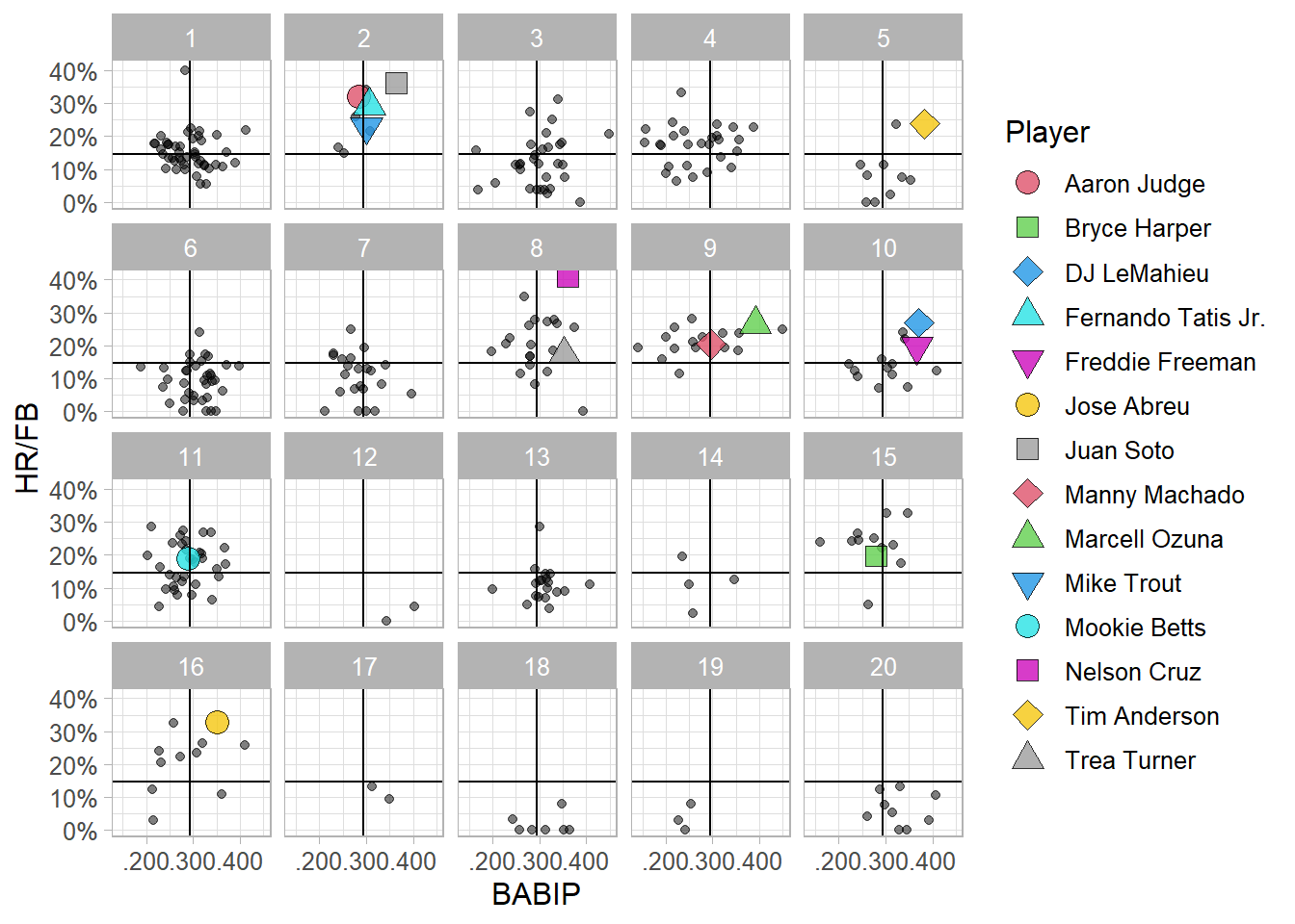
Of note, cluster 2 contains 4 of these notable players and has players with good ability to hit for average and great ability to hit for power. Judging by the players in the cluster and their results, the distributions of launch angle and exit velocity that make up this cluster must be close to ideal. Other notable positive clusters are clusters 8, 9, and 10, which each contain 2 of the most notable hitters in baseball. Clusters 18 and 19 contain some of the weaker hitters in baseball, players known largely for their defense, so the distributions that make up these clusters are not the optimal distributions of launch angle and exit velocity.
The below plot shows the overall distributions for exit velocity and launch angle for all batted balls by all players in clusters 2, 10, 18, and 19. Clusters 2 and 10 have a region of high density near 15 degrees and over 100 MPH, believed to be the sweet spot for launch angle and exit velocity. If the players in these clusters consistently hit with that launch angle and exit velocity, it makes sense that they would make up the best hitters in baseball. Note that the region of high density for cluster 2 has a slightly higher exit velocity than that for cluster 10, explaining the slight difference in player quality between the two clusters. Cluster 18 also has a region of high density around 15 degrees, but closer to 95 MPH, which explains why some of the players in that cluster might have less success. These players don’t hit the ball as hard, so they have less power. Additionally, there is a bigger region of high density above 30 degrees, which usually leads to easy fly outs for the defense. Cluster 19 has its region of highest density above 30 degrees, explaining why the cluster contains some of the weakest hitters in baseball.
in_play %>%
  left_join(kl_clusters, by = "player_name") %>%
  mutate(launch_speed = launch_speed*sd_ev+mean_ev,
         launch_angle = launch_angle*sd_la+mean_la) %>%
  filter(cluster %in% c(2,10,18,19)) %>%
  ggplot(aes(x=launch_speed, y = launch_angle)) +
  geom_density2d_filled(bins = 50, alpha = .8, na.rm = TRUE) +
  facet_wrap(~cluster) +
  theme_light() +
  theme(legend.position = "none") +
  labs(x = "Exit Velocity", y = "Launch Angle", title = "Overall Distributions of Select Clusters") +
  scale_x_continuous(limits = c(50, 120)) +
  scale_y_continuous(limits = c(-60,60))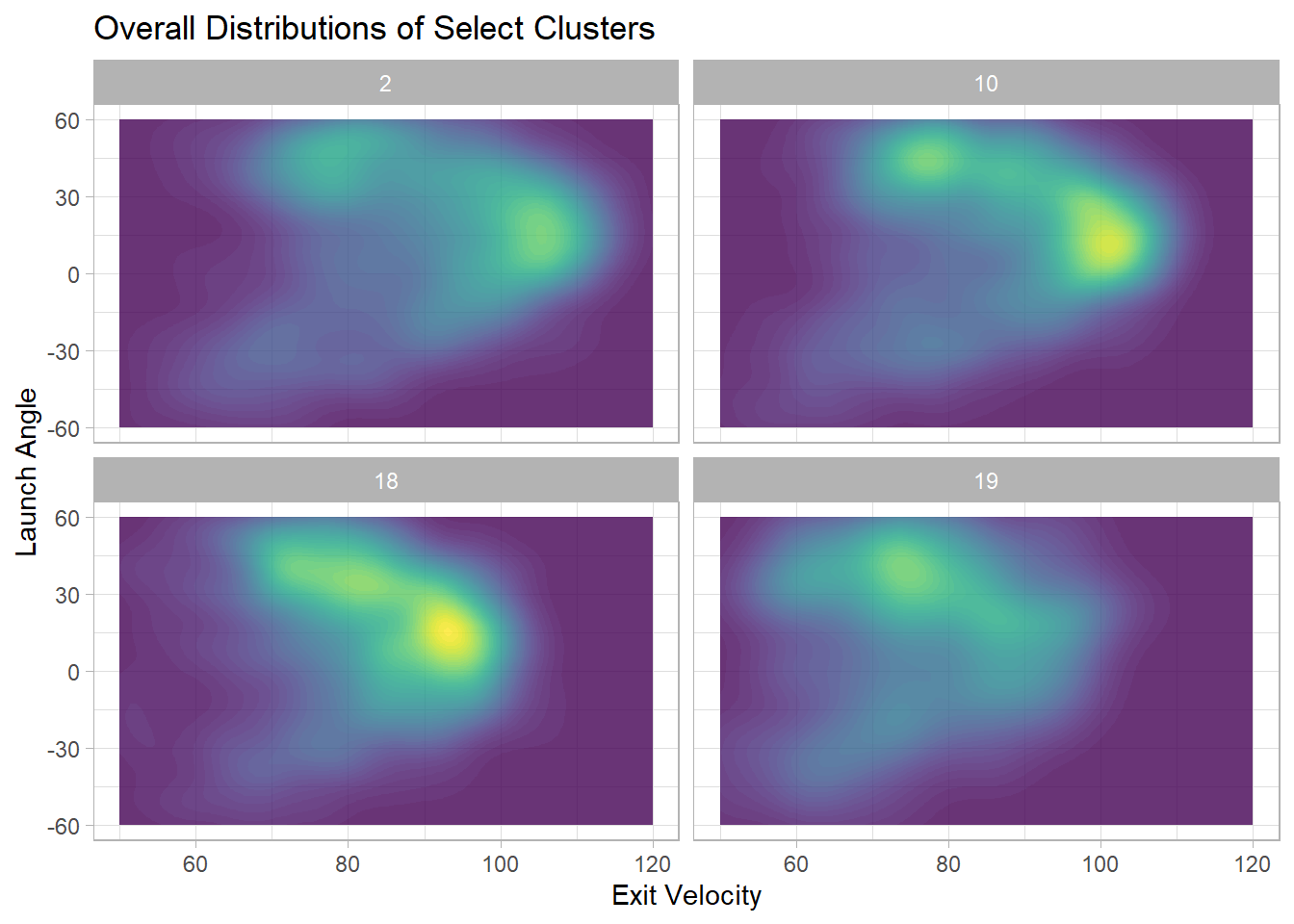
There are a variety of future applications for the clusters formed from this analysis. They could be used to have a larger sample size when predicting batter vs. pitcher matchups, to reduce the amount of information needed on a scouting report, or to identify underachieving players that belong to the same cluster as stars, prompting more work on their development.