A Bayesian Approach to Catcher Framing
In baseball, although the most important factor in whether a pitch is called a strike or not is the location of the pitch, umpires and catchers also have some effect. Some catchers are better at ``framing" a pitch, presenting it to look like it was thrown in the strike zone. Understanding which catchers are good at framing can help teams know which catchers to attempt to sign or trade for. Some umpires have slightly larger strike zones than others, so they will call more strikes on average. Knowing the strike-calling tendencies of a particular umpire would help determine how a pitcher pitches throughout a game. Thus, knowing these effects would be valuable for a team.
In this project, I fit a Bayesian mixed effect logistic regression model to achieve three goals. First, I discover which catchers are best (and worst) at framing. That is, I identify which catchers have the biggest positive (and negative) effect on whether a pitch is called a strike. Second, I find which umpires have the biggest (and smallest) strike zones, the umpires that have the biggest positive (and negative) effect on whether a pitch is called a strike. Finally, I identify whether the catcher or the umpire can make a bigger influence in whether a pitch is called a strike.
To achieve these goals, I use a data set collected from baseballsavant.com, the location of all pitch tracking data for Major League Baseball (MLB). The data set contains every pitch at which the batter didn’t swing in the 2020 MLB regular season. For each pitch, the data set contains whether the pitch was called a strike, the \(x\) and \(y\) coordinates of the pitch when it crossed the plate, the catcher on the play, and the umpire making the call. The data set includes \(133,425\) total pitches caught by \(78\) catchers and called by \(82\) umpires. For simplicity, before modeling, I convert the \(x\) and \(y\) coordinates to horizontal and vertical distances from the center of the strike zone. This adds the assumption that the strike zone is symmetric vertically and horizontally (as the rule book states it should be). This transformation makes the effects of location monotone, eliminating the need for a basis function expansion for pitch location and keeping the model simple.
library(tidyverse)
library(doParallel)
library(foreach)
library(baseballr)
library(furrr)
library(posterior)
library(ggridges)
library(xtable)
library(rstan)
library(lme4)
library(emoGG)
framing <- read_csv("framing.csv")
As stated, I fit a Bayesian logistic regression mixed effects model. The sampling model is as follows:
\[y_{ijk} | \beta_0, \beta_1, \beta_2, \beta_3, \alpha_j, \gamma_k \sim Bernoulli(\pi_{ijk})\] \[logit(\pi_{ijk}) = \beta_0 + x_{1i}\beta_1 + x_{2i}\beta_2 + x_{1i}x_{2i}\beta_3 + \alpha_j + \gamma_k\]
In this model, \(y_{ijk}\) is a binary variable indicating whether pitch \(i\) caught by catcher \(j\) was called a strike by umpire \(k\), \(\pi_{ijk}\) is the probability the pitch would be called a strike, \(\beta_0\) is the model intercept, \(x_{1i}\) is the horizontal distance from the center of the strike zone for pitch \(i\), \(x_{2i}\) is the vertical distance from the center of the strike zone for pitch \(i\), \(\beta_1\) and \(\beta_2\) are the corresponding effects for the distance from the center of the strike zone, \(\beta_3\) is an interaction effect, \(\alpha_j\) is the effect of catcher \(j\) catching the pitch, and \(\gamma_k\) is effect of umpire \(k\) calling the pitch. The \(\alpha\) parameters come from a common distribution and the \(\gamma\) parameters come from their own common distribution, giving the model a hierarchical structure.
The prior distributions are as follows:
- \(\beta_0 \sim Normal(8,3^2)\)
- \(\beta_1 \sim Normal(-5,2^2)\)
- \(\beta_2 \sim Normal(-5,2^2)\)
- \(\beta_3 \sim Normal(3, 2^2)\)
- \(\alpha_j | \tau \sim Normal(0, \frac{1}{\tau})\)
- \(\gamma_k | T \sim Normal(0, \frac{1}{T})\)
- \(\tau \sim Gamma(10,.1)\)
- \(T \sim Gamma(10,.1)\)
These prior distributions were chosen to give a reasonable shape to the strike zone, shown in the below figure.
#Plots showing the probability of a strike
make_sz_plot <- function(beta_0, beta_1, beta_2, beta_3, label){
  sz_grid <- expand.grid(horz = seq(-2.25,2.25,by = .025), vert = seq(-1.75,1.75, by = .025)) %>%
    as.data.frame()

  get_prob_strike <- function(x,y,beta_0,beta_1, beta_2, beta_3){
    plogis(beta_0 + beta_1*abs(x) + beta_2*abs(y) + beta_3*abs(x*y))
  }

  probs <- apply(sz_grid, 1, function(x) get_prob_strike(x[1], x[2],beta_0,beta_1,beta_2,beta_3))

  sz_grid$prob <- probs

  sz_grid <- sz_grid %>%
    mutate(show_point = ((horz==0 & vert==0) |
                           (horz==1 & vert==0) |
                           (horz==1 & vert==1)))

  ggplot() +
    geom_raster(sz_grid, mapping = aes(x=horz,y=vert,fill = prob)) +
    geom_polygon(mapping = aes(x=c(-1,1,1,-1,-1), y=c(-1,-1,1,1,-1)), fill = NA, col = "black", size = 1.5) +
    emoGG::geom_emoji(filter(sz_grid, show_point), mapping = aes(x=horz, y=vert), emoji = "26be") +
    geom_text(filter(sz_grid, show_point), mapping = aes(x=horz, y=vert, label = paste0(round(100*prob,2), "%")), hjust = 0, nudge_x = 0.13, size = 4.5) +
    scale_fill_gradient2(low = "royalblue3", mid = "white", high="firebrick1", midpoint = .5)  +
    theme_void() +
    theme(legend.position = "none", plot.title = element_text(hjust = 0.5, size = 18)) +
    labs(title = label)
}

make_sz_plot(8,-5,-5,3, "Prior Probability of Strike")
I gather draws from the joint posterior distribution once “by hand” (implementing my own code in R) and once using the software Stan. For the “by hand” algorithm, given the sampling model and prior distributions, I can evaluate the posterior distribution up to a proportionality constant by multiplying the joint sampling model by the joint prior distribution. The integral needed to calculate the proportionality constant cannot be evaluated in closed form, so I gather samples from the posterior distribution using sampling techniques. Choosing a disperse set of initial values for each parameter, I can iteratively update each parameter. In the algorithm, I first update \(\tau\) and \(T\), where the full conditional distributions can be derived in closed form. Given each of the \(J\) \(\alpha_j\) values and a prior distribution on \(\tau\) of \(Gamma(a,b)\), the conditional posterior distribution of \(\tau\) is a \(Gamma(a + \frac{J}{2}, b + \frac{1}{2} \sum_{j=1}^J \alpha_j^2)\) distribution. Similarly, given each of the \(K\) \(\gamma_k\) values and a prior distribution on \(T\) of \(Gamma(c,d)\), the conditional posterior distribution of \(T\) is a \(Gamma(c + \frac{K}{2}, d + \frac{1}{2} \sum_{k=1}^K \gamma_k^2)\) distribution. Then, I update each \(\alpha\) parameter. For each \(\alpha_j\), I propose a new value using a symmetric, uniform proposal distribution. I then compute the ratio of posterior densities of the proposed \(\alpha_j\) compared to the previous \(\alpha_j\) and accept the new value with probability equal to that ratio. Because the likelihood of the pitches not caught by catcher \(j\) and the densities of the other parameters are not affected by the updated \(\alpha_j\), many of the terms in the acceptance ratio cancel out and the computational burden is simplified. The below equation shows that the acceptance ratio for a new \(\alpha_1\) value (or any other \(\alpha\) parameter) simplifies to the likelihood only including the pitches caught by catcher 1 given the proposed \(\alpha_1\) and all other current parameters times the prior density of the proposed \(\alpha_1\) given the current \(\tau\) over that same product, but with the previous \(\alpha_1\) value. This ratio is further simplified by evaluating it on the log scale then exponentiating the result to find the probability of accepting a proposed draw.
\[\begin{equation} \label{eq2} \begin{split} &p(accept\:\alpha_1^*) = \frac{p(\beta_0,..., \beta_3, \alpha_1^*, \alpha_2,..., \alpha_J, \gamma_1,..., \gamma_K, \tau, T | \mathbf{y})}{p(\beta_0,..., \beta_3, \alpha_1, \alpha_2,..., \alpha_J, \gamma_1, ..., \gamma_K, \tau, T | \mathbf{y})}\\ &= \frac{k\:p(\mathbf{y} | \beta_0, ..., \beta_3, \alpha_1^*, \alpha_2,..., \alpha_J, \gamma_1,..., \gamma_K, \tau, T) p(\beta_0,..., \beta_3, \alpha_1^*, \alpha_2,..., \alpha_J, \gamma_1,..., \gamma_K, \tau, T)}{k\:p(\mathbf{y} | \beta_0,..., \beta_3, \alpha_1, \alpha_2,..., \alpha_J, \gamma_1,..., \gamma_K, \tau, T) p(\beta_0,..., \beta_3, \alpha_1, \alpha_2,..., \alpha_J, \gamma_1,..., \gamma_K, \tau, T)}\\ &= \frac{p(\mathbf{y} | \beta_0, ..., \beta_3, \alpha_1^*, \alpha_2,..., \alpha_J, \gamma_1,..., \gamma_K, \tau, T) p(\alpha_1^*|\tau)}{p(\mathbf{y} | \beta_0, ..., \beta_3, \alpha_1, \alpha_2,..., \alpha_J, \gamma_1,..., \gamma_K, \tau, T) p(\alpha_1|\tau)}\\ &= \frac{p(\mathbf{y_{.1.}} | \beta_0, ..., \beta_3, \alpha_1^*, \gamma_1,..., \gamma_K, \tau, T) p(\alpha_1^*|\tau)}{p(\mathbf{y_{.1.}} | \beta_0, ..., \beta_3, \alpha_1, \gamma_1,..., \gamma_K, \tau, T) p(\alpha_1|\tau)}\\ \end{split} \end{equation}\]
After updating all the \(\alpha\) parameters, I similarly update all the \(\gamma\) parameters. A similar cancellation occurs when evaluating the ratio of posterior densities for each proposed \(\gamma\). I then update the four \(\beta\) parameters. Because the four parameters are correlated, I update them simultaneously with a symmetric multivariate proposal distribution, using the multivariate normal distribution centered on the previous accepted draw. The same cancellation does not occur with the acceptance ratio of the \(\beta\) parameters. Because of this, the full posterior density with the proposed \(\beta\) parameters and the previous \(\beta\) parameters must be evaluated to find the acceptance ratio. The proposed parameters are accepted with probability equal to that ratio. The below code implements the algorithm.
sz_width <- 8.5/12
framing_2 <- framing %>%
  mutate(sz_height = (sz_top-sz_bot)/2) %>%
  mutate(sz_mid = sz_bot + sz_height) %>%
  mutate(dist_from_mid_vert = abs(plate_z - sz_mid)/sz_height,
         dist_from_mid_horz = abs(plate_x)/sz_width) %>%
  select(is_strike, catcher_id, umpire_name, dist_from_mid_horz,
         dist_from_mid_vert) %>%
  na.omit() %>%
  group_by(catcher_id) %>%
  filter(n() >= 500) %>%
  ungroup() %>%
  group_by(umpire_name) %>%
  filter(n() >= 500) %>%
  ungroup() %>%
  filter(dist_from_mid_vert < 4 & dist_from_mid_horz < 4)

#Create the variables that go into the model
y <- framing_2$is_strike
X1 <- framing_2$dist_from_mid_horz
X2 <- framing_2$dist_from_mid_vert
X1X2 <- X1*X2
X3 <- as.numeric(as.factor(framing_2$catcher_id))
X4 <- as.numeric(as.factor(framing_2$umpire_name))

#By hand fit

#Proposal covaraince matrix for beta parameters
cov_mat <- matrix(c(.01,-.003,-.004,.002,
                    -.003,.004,.0008,-.001,
                    -.004,.0008,.006,-.001,
                    .002,-.001,-.001,.002), ncol =4, byrow = TRUE)

#Function that does one chain
do_mcmc <- function(nruns = 2000,
                    starting_beta = c(8,-5,-5,3),
                    starting_alpha = c(0.033,0.097,-0.115,0.118,-0.143,0.076,-0.095,-0.179,0.024,-0.015,-0.093,-0.008,-0.054,0.038,0.031,0.088,0.239,-0.059,0.043,0.034,-0.13,0.145,0.195,0.144,0.089,0.036,-0.114,0.066,0.047,0.243,0.074,0.036,-0.144,0.022,0.141,0.084,-0.05,0.043,-0.13,0.026,-0.166,-0.042,0.042,-0.092,-0.071,0.226,0.01,-0.128,-0.075,-0.015,-0.167,0.022,0.055,-0.172,-0.151,0.064,-0.166,0.071,-0.101,0.007,-0.052,-0.043,-0.021,0.094,-0.084,-0.229,0.095,0.002,0.103,0.025,0.069,0.053,0.094,0.007,-0.066,-0.09,-0.122,0.154),
                    starting_gamma = c(-0.205,0.358,-0.125,-0.105,-0.018,-0.275,-0.019,0.105,-0.058,0.189,0.055,-0.092,-0.075,-0.177,0.112,0.012,0.087,0.029,-0.124,-0.048,-0.073,-0.134,0.16,-0.051,0.051,0.291,0.407,-0.178,-0.028,0.043,0.068,-0.068,-0.145,-0.067,-0.023,0.053,-0.046,-0.014,-0.057,-0.103,0.006,-0.08,-0.176,-0.155,0.11,-0.014,0.424,0.058,-0.035,-0.25,-0.047,0.004,-0.075,-0.176,-0.021,0.024,-0.098,0.288,-0.133,0.107,0.233,-0.219,-0.076,0.175,0.173,-0.076,0.196,0.013,-0.039,0.16,-0.131,0.056,-0.05,0.006,0.064,0.011,-0.138,-0.091,-0.091,0.119,0.211,0.058),
                    starting_tau = 100,
                    starting_T1 = 100,
                    m0 = 8,
                    v0 = 3,
                    m1 = -5,
                    v1 = 2,
                    m2 = -5,
                    v2 = 2,
                    m3 = 3,
                    v3 = 2,
                    a = 10,
                    b = .1,
                    c = 10,
                    d = .1,
                    d_alpha = .2,
                    d_gamma = .2,
                    d_beta = cov_mat/10
){
  beta <- matrix(NA, nruns, 4)
  alpha <- matrix(NA, nruns, max(X3))
  gamma <- matrix(NA, nruns, max(X4))
  tau <- matrix(NA, nruns, 1)
  T1 <- matrix(NA, nruns, 1)

  beta[1,] <- starting_beta
  alpha[1,] <- starting_alpha
  gamma[1,] <- starting_gamma

  tau[1] <- starting_tau
  T1[1] <- starting_T1

  inv_logit<- function(a){
    exp(a)/(exp(a)+1)
  }

  log_lik_rat <- function(beta0_a, beta1_a, beta2_a, beta3_a, alpha_a, gamma_a, tau_a, T1_a,
                          beta0_b, beta1_b, beta2_b, beta3_b, alpha_b, gamma_b, tau_b, T1_b){
    to_add_in <- dbinom(y,
                        1,
                        inv_logit(beta0_a + beta1_a*X1 + beta2_a*X2 + beta3_a*X1X2 + alpha_a[X3] + gamma_a[X4]),
                        log = TRUE) -
      dbinom(y,
             1,
             inv_logit(beta0_b + beta1_b*X1 + beta2_b*X2 + beta3_b*X1X2 + alpha_b[X3] + gamma_b[X4]),
             log = TRUE)
    res <- dnorm(beta0_a, m0, v0, log = TRUE) +
      dnorm(beta1_a, m1, v1, log = TRUE) +
      dnorm(beta2_a, m2, v2, log = TRUE) +
      dnorm(beta3_a, m3, v3, log = TRUE) +
      sum(dnorm(alpha_a, 0, 1/sqrt(tau_a), log = TRUE)) +
      sum(dnorm(gamma_a, 0, 1/sqrt(T1_a), log = TRUE)) +
      dgamma(tau_a, a, b, log = TRUE) +
      dgamma(T1_a, c, d, log = TRUE) -
      dnorm(beta0_b, m0, v0, log = TRUE) -
      dnorm(beta1_b, m1, v1, log = TRUE) -
      dnorm(beta2_b, m2, v2, log = TRUE) -
      dnorm(beta3_b, m3, v3, log = TRUE) -
      sum(dnorm(alpha_b, 0, 1/sqrt(tau_b), log = TRUE)) -
      sum(dnorm(gamma_b, 0, 1/sqrt(T1_b), log = TRUE)) -
      dgamma(tau_b, a, b, log = TRUE) -
      dgamma(T1_b, c, d, log = TRUE) +
      sum(to_add_in, na.rm = TRUE)
    res
  }

  log_lik_alpha <- function(j,beta0_a, beta1_a, beta2_a, beta3_a, alpha_a, gamma_a, tau_a, T1_a,
                            beta0_b, beta1_b, beta2_b, beta3_b, alpha_b, gamma_b, tau_b, T1_b){
    to_use <- which(X3 == j)
    to_add_in <- dbinom(y[to_use],
                        1,
                        inv_logit(beta0_a + beta1_a*X1[to_use] + beta2_a*X2[to_use] + beta3_a*X1X2[to_use] + alpha_a[X3[to_use]] + gamma_a[X4[to_use]]),
                        log = TRUE) -
      dbinom(y[to_use],
             1,
             inv_logit(beta0_b + beta1_b*X1[to_use] + beta2_b*X2[to_use] + beta3_b*X1X2[to_use] + alpha_b[X3[to_use]] + gamma_b[X4[to_use]]),
             log = TRUE)
    res <- sum(dnorm(alpha_a, 0, 1/sqrt(tau_a), log = TRUE)) -
      sum(dnorm(alpha_b, 0, 1/sqrt(tau_b), log = TRUE)) +
      sum(to_add_in, na.rm = TRUE)
    res
  }

  log_lik_gamma <- function(j,beta0_a, beta1_a, beta2_a, beta3_a, alpha_a, gamma_a, tau_a, T1_a,
                            beta0_b, beta1_b, beta2_b, beta3_b, alpha_b, gamma_b, tau_b, T1_b){
    to_use <- which(X4 == j)
    to_add_in <- dbinom(y[to_use],
                        1,
                        inv_logit(beta0_a + beta1_a*X1[to_use] + beta2_a*X2[to_use] + beta3_a*X1X2[to_use] + alpha_a[X3[to_use]] + gamma_a[X4[to_use]]),
                        log = TRUE) -
      dbinom(y[to_use],
             1,
             inv_logit(beta0_b + beta1_b*X1[to_use] + beta2_b*X2[to_use] + beta3_b*X1X2[to_use] + alpha_b[X3[to_use]] + gamma_b[X4[to_use]]),
             log = TRUE)
    res <- sum(dnorm(gamma_a, 0, 1/sqrt(T1_a), log = TRUE)) -
      sum(dnorm(gamma_b, 0, 1/sqrt(T1_b), log = TRUE)) +
      sum(to_add_in, na.rm = TRUE)
    res
  }

  log_lik_beta <- function(beta0_a, beta1_a, beta2_a, beta3_a, alpha_a, gamma_a, tau_a, T1_a,
                           beta0_b, beta1_b, beta2_b, beta3_b, alpha_b, gamma_b, tau_b, T1_b){
    to_add_in <- dbinom(y,
                        1,
                        inv_logit(beta0_a + beta1_a*X1 + beta2_a*X2 + beta3_a*X1X2 + alpha_a[X3] + gamma_a[X4]),
                        log = TRUE) -
      dbinom(y,
             1,
             inv_logit(beta0_b + beta1_b*X1 + beta2_b*X2 + beta3_b*X1X2 + alpha_b[X3] + gamma_b[X4]),
             log = TRUE)
    res <- dnorm(beta0_a, m0, v0, log = TRUE) +
      dnorm(beta1_a, m1, v1, log = TRUE) +
      dnorm(beta2_a, m2, v2, log = TRUE) +
      dnorm(beta3_a, m3, v3, log = TRUE)  -
      dnorm(beta0_b, m0, v0, log = TRUE) -
      dnorm(beta1_b, m1, v1, log = TRUE) -
      dnorm(beta2_b, m2, v2, log = TRUE) -
      dnorm(beta3_b, m3, v3, log = TRUE) +
      sum(to_add_in, na.rm = TRUE)
    res
  }

  p <- ncol(alpha)
  q <- ncol(gamma)

  current_time <- as.numeric(Sys.time())


  for(i in 2:nruns){
    #Update tau
    tau[i] <- rgamma(1, a + p/2, b + 1/2*sum((alpha[i-1,])^2))

    #Update T1
    T1[i] <- rgamma(1, c+q/2, d + 1/2*sum((gamma[i-1,])^2))

    #Update alpha
    alpha_vec <- alpha[i-1,]
    for(j in 1:ncol(alpha)){
      prop <- alpha_vec[j] + runif(1,-d_alpha, d_alpha)
      prop_vec <- alpha_vec
      prop_vec[j] <- prop
      prob_accept <-  exp(log_lik_alpha(j, beta0_a = beta[i-1,1], beta1_a = beta[i-1,2],
                                        beta2_a = beta[i-1,3], beta3_a = beta[i-1,4],
                                        alpha_a = prop_vec, gamma_a = gamma[i-1,],
                                        tau_a = tau[i], T1_a = T1[i],
                                        beta0_b = beta[i-1,1], beta1_b = beta[i-1,2],
                                        beta2_b = beta[i-1,3], beta3_b = beta[i-1,4],
                                        alpha_b = alpha_vec, gamma_b = gamma[i-1,],
                                        tau_b = tau[i], T1_b = T1[i]))
      alpha_vec[j] <- ifelse(prob_accept > runif(1), prop_vec[j], alpha_vec[j])
    }
    alpha[i,] <- alpha_vec

    #Update gamma
    gamma_vec <- gamma[i-1,]
    for(j in 1:ncol(gamma)){
      prop <- gamma_vec[j] + runif(1,-d_gamma, d_gamma)
      prop_vec <- gamma_vec
      prop_vec[j] <- prop
      prob_accept <-  exp(log_lik_gamma(j, beta0_a = beta[i-1,1], beta1_a = beta[i-1,2],
                                        beta2_a = beta[i-1,3], beta3_a = beta[i-1,4],
                                        alpha_a = alpha[i,], gamma_a = prop_vec,
                                        tau_a = tau[i], T1_a = T1[i],
                                        beta0_b = beta[i-1,1], beta1_b = beta[i-1,2],
                                        beta2_b = beta[i-1,3], beta3_b = beta[i-1,4],
                                        alpha_b = alpha[i,], gamma_b = gamma_vec,
                                        tau_b = tau[i], T1_b = T1[i]))
      gamma_vec[j] <- ifelse(prob_accept > runif(1), prop_vec[j], gamma_vec[j])
    }
    gamma[i,] <- gamma_vec


    #Update betas
    prop <- mvtnorm::rmvnorm(1, beta[i-1,], d_beta)
    prob_accept <-  exp(log_lik_beta(beta0_a = prop[1], beta1_a = prop[2],
                                     beta2_a = prop[3], beta3_a = prop[4],
                                     alpha_a = alpha[i,], gamma_a = gamma[i,],
                                     tau_a = tau[i], T1_a = T1[i],
                                     beta0_b = beta[i-1,1], beta1_b = beta[i-1,2],
                                     beta2_b = beta[i-1,3], beta3_b = beta[i-1,4],
                                     alpha_b = alpha[i,], gamma_b = gamma[i,],
                                     tau_b = tau[i], T1_b = T1[i]))

    acc <- prob_accept > runif(1)
    beta[i,1] <- ifelse(acc, prop[1], beta[i-1,1])
    beta[i,2] <- ifelse(acc, prop[2], beta[i-1,2])
    beta[i,3] <- ifelse(acc, prop[3], beta[i-1,3])
    beta[i,4] <- ifelse(acc, prop[4], beta[i-1,4])
  }
  tot_time <- as.numeric(Sys.time())-current_time
  list(beta = beta, alpha = alpha, gamma = gamma, tau = tau, T1 = T1, tot_time = tot_time)
}
nCores <- 3
registerDoParallel(nCores)
nSub <- 3
system.time({result <- foreach(i = 1:nSub) %dopar% {
do_mcmc(nruns = 15000, starting_alpha = rnorm(max(X3),0,.2),
starting_gamma = rnorm(max(X4),0,.2))
}})Using this algorithm, I gather 15,000 posterior draws for each parameter, of which I discard the first 5,000 as burn in. I run this algorithm with three chains, leading to 30,000 total posterior draws. Using these draws, I can evaluate which catchers are best at framing and which umpires have the biggest strike zones.
keep <- 5001:15000
beta <- map(1:3, function(x) result[[x]]$beta[keep,]) %>% plyr::ldply(data.frame) %>% as.matrix()
alpha <- map(1:3, function(x) result[[x]]$alpha[keep,]) %>% plyr::ldply(data.frame) %>% as.matrix()
gamma <- map(1:3, function(x) result[[x]]$gamma[keep,]) %>% plyr::ldply(data.frame) %>% as.matrix()
tau <- c(sapply(1:3, function(x) result[[x]]$tau[keep]))
T1 <- c(sapply(1:3, function(x) result[[x]]$T1[keep]))
The first question in this analysis relates to which catchers are the best and worst at framing pitches. A catcher that has positive value in framing pitches will have a positive corresponding \(\alpha\) effect. The below plot in Figure shows the posterior distributions of the effects of the top and bottom 10 catchers in framing. Omar Narvaez, Yasmani Grandal, and Austin Barnes appear to be the three best catchers at framing, based on the model of the 2020 data. The point estimate for the effect of Narvaez as a catcher is .227 (95% Monte Carlo CI between .225 and .229), with a 95% credible interval between .091 and .369. Additionally, the probability that Narvaez has the biggest framing effect is .23 (95% Monte Carlo CI between .219 and .241).
catchers <- levels(as.factor(framing_2$catcher_id))
catchers_names <- sapply(catchers, function(x){
  baseballr::playername_lookup(x) %>%
    mutate(name = paste(name_first, name_last)) %>%
    pull(name)
}) %>% as.character()
colnames(alpha) <- catchers_names
top_alpha <- colMeans(alpha) %>% sort(decreasing = TRUE) %>% head(10) %>% names()
bot_alpha <- colMeans(alpha) %>% sort(decreasing = TRUE) %>% tail(10) %>% names()
alpha[,c(top_alpha,bot_alpha)] %>%
as.data.frame() %>%
pivot_longer(everything()) %>%
group_by(name) %>%
mutate(m = mean(value)) %>%
ungroup() %>%
ggplot(aes(x=value, y = fct_reorder(name, value), fill = m)) +
ggridges::geom_density_ridges(quantile_lines = TRUE, quantiles = 2, scale = 1.5, show.legend = FALSE) +
theme_light() +
scale_fill_gradient2(low = "blue", mid = "white", high = "red") +
labs(x= "Effect", y = "", title = "Best and Worst Framers") +
theme(panel.grid.major = element_blank(), panel.grid.minor = element_blank())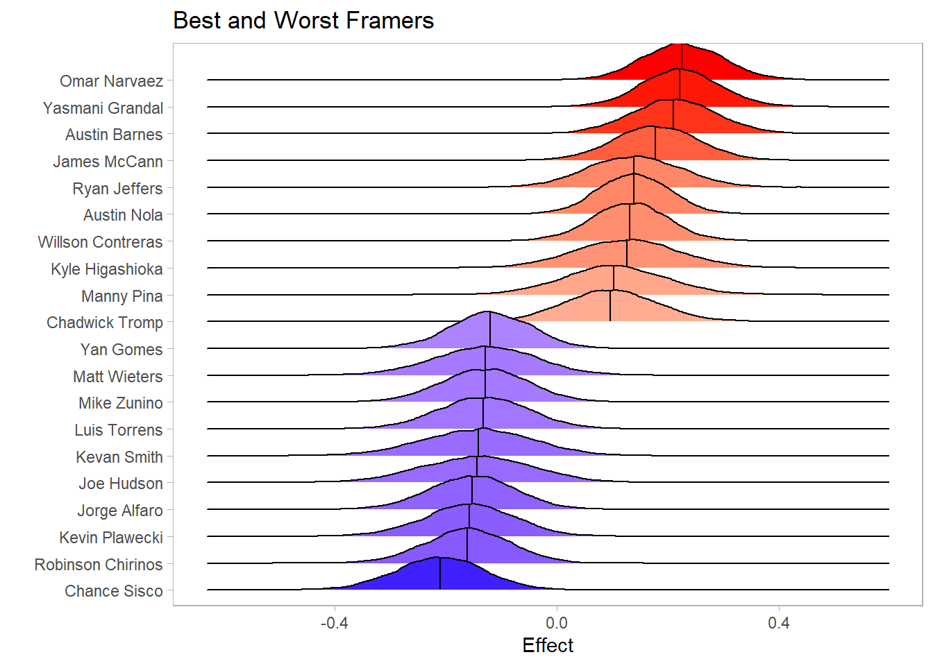
The second question in this analysis relates to which umpires have the biggest and smallest strike zones. An umpire that has a bigger strike zone will have a positive corresponding \(\gamma\) effect. The below plot shows the posterior distributions of the effects of the umpires with the biggest and smallest strike zones. Lance Barrett, Ed Hickox, and Adam Hamari appear to have the biggest strike zones, based on the model of the 2020 data. The point estimate for the effect of having Barrett as an umpire is .396 (95% Monte Carlo CI between .394 and .399), with a 95% credible interval between .237 and .552. Additionally, the probability that Barrett has the biggest strike zone is .423 (95% Monte Carlo CI between .408 and .438).
umpires_names <- levels(as.factor(framing_2$umpire_name))
colnames(gamma) <- umpires_names

top_gamma <- colMeans(gamma) %>% sort(decreasing = TRUE) %>% head(10) %>% names()
bot_gamma <- colMeans(gamma) %>% sort(decreasing = TRUE) %>% tail(10) %>% names()

gamma[,c(top_gamma,bot_gamma)] %>%
  as.data.frame() %>%
  pivot_longer(everything()) %>%
  group_by(name) %>%
  mutate(m = mean(value)) %>%
  ungroup() %>%
  ggplot(aes(x=value, y = fct_reorder(name, value), fill = m)) +
  ggridges::geom_density_ridges(quantile_lines = TRUE, quantiles = 2, scale = 1.5, show.legend = FALSE) +
  theme_light() +
  scale_fill_gradient2(low = "blue", mid = "white", high = "red") +
  labs(x= "Effect", y = "", title = "Biggest and Smallest Umpire Strike Zones") +
  theme(panel.grid.major = element_blank(), panel.grid.minor = element_blank())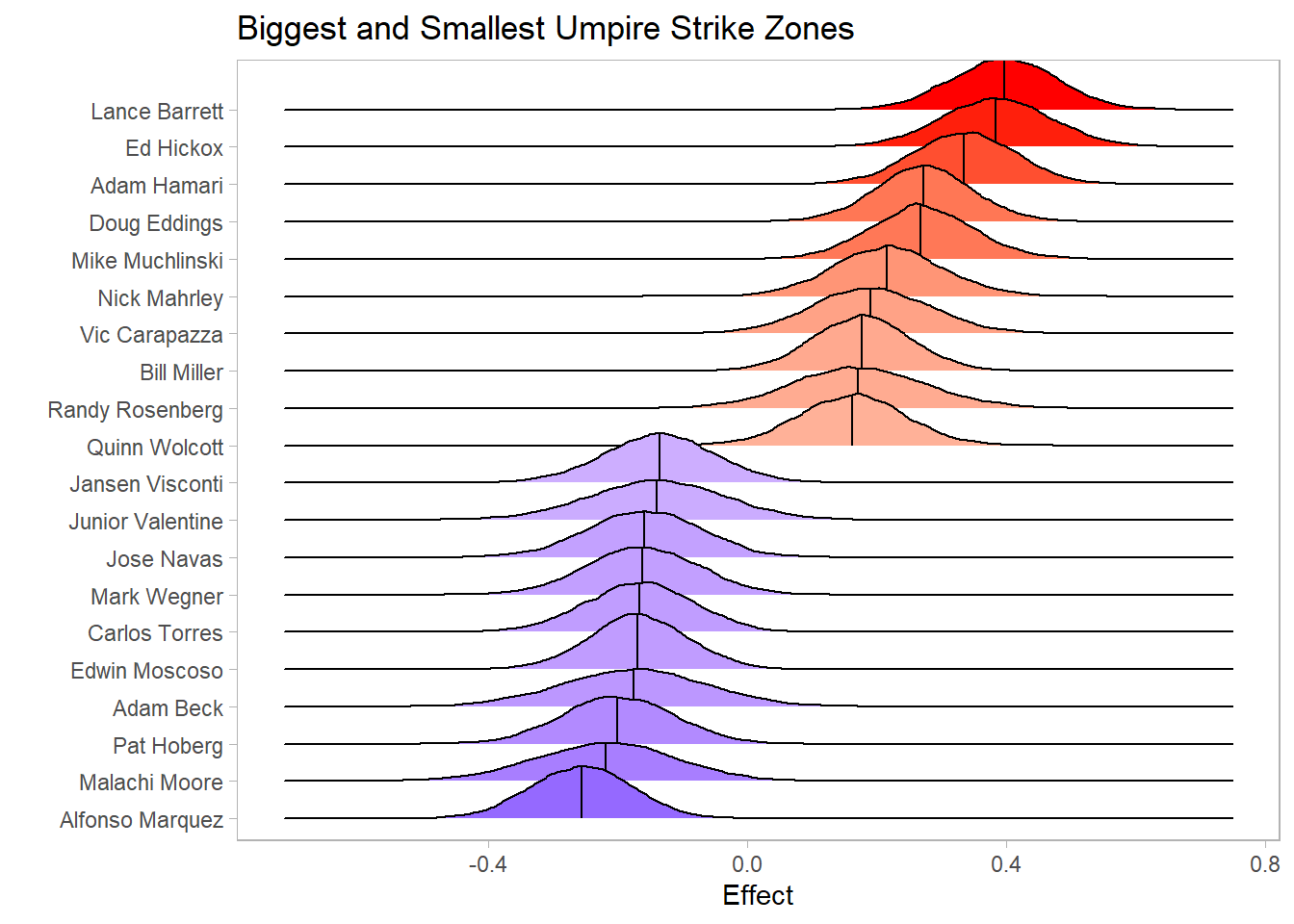
Unfortunately, these effects are not simple to understand. Although they make clear which catchers are the best at framing and which umpires have the biggest strike zones, they do not make clear the amount of value a catcher can add or how big the difference between two umpires can be. The below plots show how the probabilities of a pitch being called a strike change with different catchers and umpires (using the Bayesian estimator under squared error loss for each effect to calculate the probabilities). The calls of pitches in the center of the rule book strike zone or at the edge of the strike zone don’t vary too much with the catcher and umpire, but the calls of pitches at the corners of the strike zone can be impacted more by the catcher and umpire. With an average catcher and umpire (i.e., no catcher or umpire effect), the probability that a pitch on the corner of the strike zone is called a strike is about 25%. With the top catcher (Narvaez) and the umpire with the biggest strike zone (Barrett), that probability increases to about 39%. With the worst catcher and the umpire with the smallest strike zone, that probability drops to 17.5%. Note that the true strike zone estimated by the model does not match the rectangular strike zone defined by the MLB rulebook. Although this may seem odd, past research by Eli Ben-Porat (https://tht.fangraphs.com/rethinking-the-strike-zone-its-not-a-square/) supports the notion that the true strike zone is much rounder than it is supposed to be.
make_sz_plot(12, -7.95,-9.16,4.03, "Probability of Strike \n Average Catcher, Average Umpire Zone")
make_sz_plot(12+.23+.4, -7.95,-9.16,4.03, "Probability of Strike \n Top Catcher, Biggest Umpire Zone")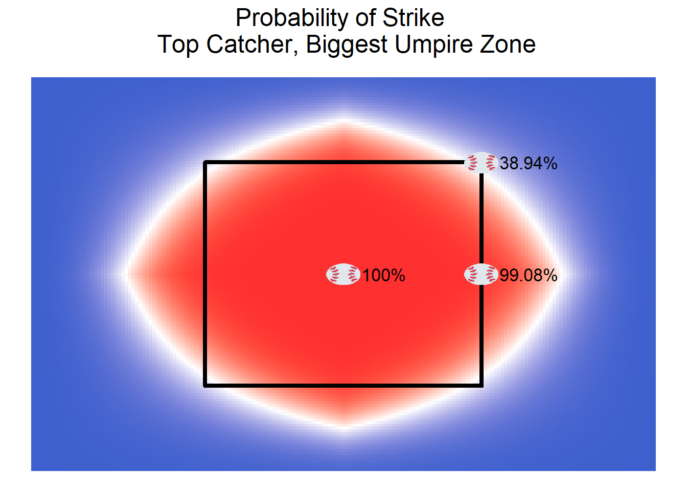
make_sz_plot(12-.21-.26, -7.95,-9.16,4.03, "Probability of Strike \n Worst Catcher, Smallest Umpire Zone")
To go beyond percentages and further explore how much value a good framing catcher can add to a team’s success over the course of a season, the original data combined with the samples from the posterior distribution can be used to simulate how many strikes a catcher may add above what actually occurred on the pitches. To calculate this value, I first sample 1,000 pitches from the data set and 1,000 draws from the posterior distribution. For each pitch, I use one set of posterior parameter estimates to estimate the probability that the pitch would be called a strike for each catcher, then simulate whether the pitch would be called a strike for each catcher by sampling from a Bernoulli distribution with those probabilities. Doing this for each pitch gives the number of strikes the catcher would have had called in those 1,000 pitches. Subtracting the actual number of strikes called yields the strikes the catcher added per 1,000 pitches in that simulation. Repeating that process 1,000 times and taking the average leads to a catcher’s Expected Strikes Added from Framing per 1,000 pitches (xSAF/1000). Past research by Tom Tango (http://tangotiger.com/index.php/site/wowy-framing-part-3-of-n-run-value-of-a-called-strike) has shown that 8 strikes added is equal in value to 1 run added/prevented, so dividing xSAF/1000 by 8 leads to Expected Runs Added from Framing per 1,000 pitches (xRAF/1000). Using the precedent that 10 runs added/prevented is equal in value to 1 win added, so dividing xRAF/1000 by 10 leads to Expected Wins Added from Framing per 1,000 pitches (xWAF/1000). Because a typical starting catcher will catch around 5,000 callable pitches per season, the best catchers should add about a win of value above the average catcher through their framing abilities alone. In any given 1,000 pitches, a catcher may add more or less value, shown by the lower and upper bounds in Table the table, but on the average, the best framing catchers should add substantial value.
plan(multiprocess, workers = 3)
res <- future_map_dfr(sample(1:length(beta0), 10000, replace = TRUE), function(x){
  x <- get_strikes_per_1000(beta0[x], beta1[x],
                            beta2[x], beta3[x],
                            alpha[x,], gamma[x,])
  names(x) <- catchers_names
  x %>% t() %>% as.data.frame()
}, .progress = TRUE)

res %>%
  pivot_longer(everything()) %>%
  group_by(name) %>%
  summarize(xSAF = mean(value),
            Lower = quantile(value, .1),
            Upper = quantile(value, .9)) %>%
  arrange(desc(abs(xSAF))) %>%
  head(10) %>%
  arrange(desc(xSAF)) %>%
  mutate(xRAF = xSAF*.125) %>%
  mutate(xWAF = xRAF/10)  %>%
rename(Catcher = name)| Catcher | xSAF/1000 | Lower | Upper | xRAF/1000 | xWAF/1000 |
|---|---|---|---|---|---|
| Omar Narvaez | 13.66 | -2.00 | 29.00 | 1.71 | 0.17 |
| Yasmani Grandal | 13.43 | -2.00 | 29.00 | 1.68 | 0.17 |
| Austin Barnes | 12.63 | -3.00 | 28.00 | 1.58 | 0.16 |
| James McCann | 10.41 | -5.00 | 26.00 | 1.30 | 0.13 |
| Kevan Smith | -9.07 | -25.00 | 7.00 | -1.13 | -0.11 |
| Joe Hudson | -9.36 | -26.00 | 7.00 | -1.17 | -0.12 |
| Jorge Alfaro | -9.79 | -25.00 | 6.00 | -1.22 | -0.12 |
| Kevin Plawecki | -10.23 | -26.00 | 5.00 | -1.28 | -0.13 |
| Robinson Chirinos | -10.54 | -26.00 | 5.00 | -1.32 | -0.13 |
| Chance Sisco | -13.59 | -29.00 | 2.00 | -1.70 | -0.17 |
The final question of interest in this analysis is whether catchers or umpires have a bigger effect on whether a pitch is called a strike. This question can be answered by analyzing the posterior distributions of \(\tau\) and \(T\). If \(\tau\) is larger than \(T\), the precision of the distribution of the effects of catchers is larger than the precision of the distribution of the effects of umpires. This means that on average, the effect of catchers will be closer to 0, so catchers have a smaller effect on whether a pitch is called as strike than umpires do. This appears to be the case in the model of the 2020 data. The probability that \(\tau\) is larger than \(T\) is .913 (Monte Carlo CI between .902 and .923). Thus, umpires tend to have a larger impact on whether a pitch is called a strike than catchers do. This makes some intuitive sense, as umpires have the final decision of whether a pitch is a strike or not. Additionally, the effect of the umpire with the biggest strike zone appears to be twice as large as the effect of the best framing catcher.
Thus, the model identified Omar Narvaez as the top framing catcher in baseball, adding about a win in value over an average catcher. The model also identified Lance Barrett as the umpire with the biggest strike zone in the 2020 season and found that the umpire effects were more variable than the catcher effects. One area where the analysis could be improved upon would be to allow more flexibility in the shape of the strike zone through not assuming a symmetric strike zone and using basis function expansions to allow different location effects. The true shape of the strike zone was not a main focus of this analysis, but future research on its true shape may prove useful for improving this catcher framing model.